
HTML report
*The interpretation of the HTML report is only available in EN.
SAW count and SAW realign pipelines will output an interactive report <SN>.report.html . The contents of the HTML report file will vary depending on the pipeline and parameters used but generally follow a similar format across runs.
On this page, we partly demonstrate the reports of
- a mouse brain sample from Stereo-seq T FF V1.3,
- a mouse lung tissue sample from Stereo-seq N FFPE V1.0,
- and a mouse spleen tissue sample from Stereo-CITE T FF V1.1.
From SAW 8.2, the HTML report interface has undergone a significant UI upgrade, along with optimizations to the hierarchical structure and information layout. For the first time, results are presented from a multi-omics and multi-modal perspective, with primary navigation tabs such as Gene, Protein, Microbe, and Image to integrate and organize information effectively.
Gene
Summary
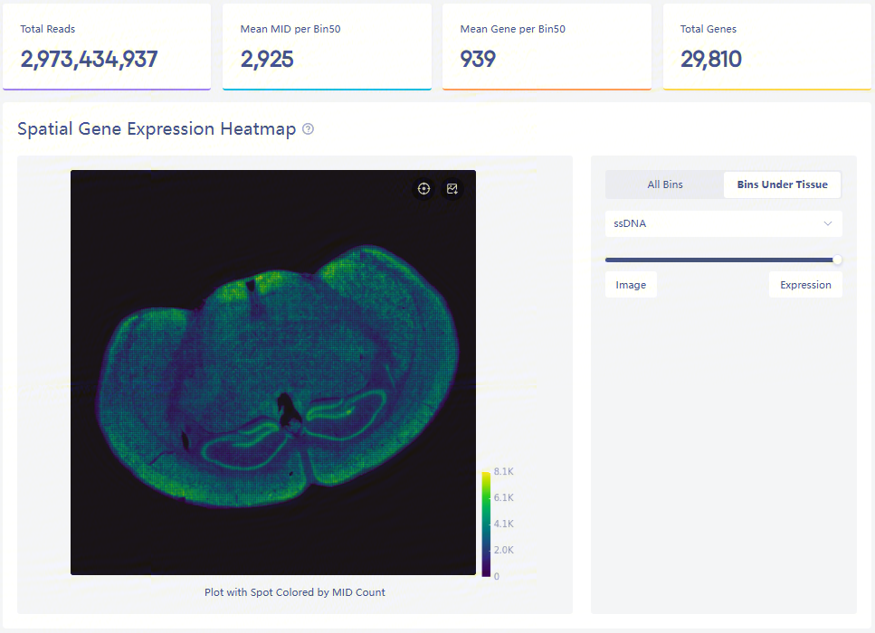
Expression heatmap and four key metrics
.png)
Display of microscope image
The spatial gene expression distribution plot, containing all bins and bins under tissue, on the left, shows MID count at each bin50.
Total Reads is the amount of total sequencing reads of input FASTQs. Mean MID per Bin50 and Mean Gene per Bin50 represent the mean MID and gene type counts at each bin50 under the detected tissue region. Total Genes is the number of gene types from all bins.
Gene key metrics
.png)
Details and sunburst plot of key metrics
Gene key metrics of the data are listed:
| Metric | Description |
|---|---|
| Total Reads (Gene) | Number of total transcriptome sequenced reads. |
| Valid CID Reads | Number of reads with CID (coordinate ID) sequences matched to the Stereo-seq chip. |
| Invalid CID Reads | Number of reads with CID (coordinate ID) sequences not matched to the Stereo-seq chip. |
| Clean Reads | Number of reads that have passed the filtering steps. |
| Non-Relevant Short Reads | Number of non-relevant short reads, i.e. the reads contain specific sequences of chip DNB, or have a length of less than 30bp after the removal of adapters and polyA tails. |
| Discarded MID Reads | Number of reads with invalid MID (Molecular ID), i.e. MID sequences contain Ns or more than 1 low quality base (Q-score < 30). |
| Confidently Mapped Reads | Number of reads mapped to a single region on the genome with high confidence, i.e. this item usually includes the reads uniquely mapped to the genome, as well as the best alignment among multi-mapped reads. It is affected by the setting of the --uniquely-mapped-only option. |
| Transcriptome | Number of reads that can be mapped to the transcripts of a single gene. |
| Unique Reads | Number of annotated reads with unique gene ID, CID (Coordinate ID), MID (Molecule ID), i.e. the reads are not PCR duplicated |
| Sequencing Saturation | Number of annotated reads corrected by MAPQ with duplicated MIDs. |
| Unannotated Reads | Number of reads that cannot be mapped to the transcripts of any gene or only a single gene. |
| Multi-Mapped Reads | Number of reads that can be mapped to multiple positions on the genome with the same high confidence level, excluding the best matching ones. It is affected by the setting of the --uniquely-mapped-only option. |
| Unmapped Reads | Number of reads that cannot be mapped to the reference genome. |
| rRNA Reads | Number of reads mapped to specific rRNA regions, according to the input reference. |
Annotation
Metrics of reads to be annotated by GTF/GFF files.
| Metric | Description |
|---|---|
| Exonic | Number of reads that can be confidently mapped to an exonic region and on the same strand of the gene. |
| Intronic | Number of reads that can be confidently mapped to an intronic region and on the same strand of the gene. |
| Intergenic | Number of reads mapped to an intergenic region and on the same strand of the genome. |
| Antisense | Number of reads mapped to the transcriptome but on the opposite strand of the annotated gene. |
Tissue region
Metrics related to tissue coverage are listed:
| Metric | Description |
|---|---|
| Tissue Area | Detected tissue area in mm². |
| MID Under Tissue | MID count under tissue. The detected tissue region depends on the automatic/manual tissue segmentation. |
| Fraction MID in Spots Under Tissue | Fraction of MID under tissue over total unique reads (Number of MID Under Tissue / Unique Reads). |
Sequencing saturation
.png)
Sequencing saturation curves
The saturation analysis in the HTML report can assess the overall quality of the sequencing data. In order to improve calculation efficiency, small samples are randomly selected from successfully annotated reads in the bin20 or bin50 dimension. Therefore, the results of multiple runs of the same data may vary slightly. The formulas may not be identical, but the general shape of the curve is consistent.
- Figure 1: As the number of random samples increases, the gene median in the bin20 dimension gradually increases.
- Figure 2: Curves fitted based on Unique Reads data from randomly sampled samples.
- Figure 3: Statistics of Unique Reads (reads with unique CID, geneName and MID) in the sampled samples, saturation value = 1-(Unique Reads)/(Total Annotated Reads), as the sampling volume increases, the fitting curve becomes near-flat, indicating that the data tends to be saturated. Whether to add additional tests depends on the overall project design and sample conditions. For example, it is recommended that additional tests be performed on precious samples. The threshold value of 0.8 in the report serves as a reminder for recommended guidance.
The x-axis of the three graphs is the same, and the y-axis is divided into saturation value, gene median, and number of Unique Reads.
Sample information
This item displays the basic information of the input datasets.
| Metric | Description |
|---|---|
| Sample ID | ID for this HTML report. |
| Organism | Organism information of the sample. |
| Tissue | Tissue type of the sample. |
| Reference | Reference used for reads alignment and annotation. |
| Kit Version | Version of the Stereo-seq product kit. |
| Sequencing Type | Sequencing type for the Stereo-seq product kit. |
| Stereo-seq Chip SN | The serial number of the Stereo-seq chip. |
| FASTQ | Detailed information of input FASTQ files. |
Square Bin
This page contains statistics, plots, clustering, UMAP, and differential expression analysis results, at bin dimension. Results come from the analysis based on <SN>.tissue.gef file. This sub-page will display the analysis result of bin20 and bin50 by default, which depends on --custom-bin-size when you start SAW count/realign.
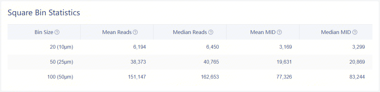
Statistics
.png)
Statistics of bins under tissue-coverage region
The above table records the statistics for bin20, bin50, and bin100:
| Item | Description |
|---|---|
| Bin Size | A unit bin, referred to as an expression spot, is used to aggregate DNBs (on the Stereo-seq chip) within a square region (i.e., bin20 = 20 x 20 DNBs). |
| Mean Reads (per bin) | Average number of sequenced reads within a binN (under detected tissue region). |
| Median Reads (per bin) | Median number of sequenced reads within a binN (under detected tissue region). |
| Mean Gene Type (per bin) | Average number of gene type within a binN (under detected tissue region). |
| Median Gene Type (per bin) | Median number of gene type within a binN (under detected tissue region). |
| Mean MID (per bin) | Average number of MID count within a binN (under detected tissue region). |
| Median MID (per bin) | Median number of MID count within a binN (under detected tissue region). |
Plots
.png)
Distribution plots of MID and gene type
Violin plots show the distribution of deduplicated MID count and gene types in each bin.
Clustering & UMAP
.png)
Leiden clustering and UMAP projection
Clustering is performed based on SN.tissue.gef using the Leiden algorithm. UMAP projections are performed based on SN.tissue.gef and colored by automated clustering. The same color is assigned to spots that are within a shorter distance and with similar gene expression profiles.
Note that this part will present the results of certain large-sized Stereo-seq chips through downsampling to reduce file size, minimize spot overlap, and ensure a smooth display, especially in cases where there are an excessive number of spots to visualize.
We discovered that when the number of spots in the graph exceeds one million, it significantly impacts both the visual mapping quality and file reading performance. Consequently, we implemented downsampling. A smaller bin size requires a greater number of spots for effective mapping. For detailed information regarding the downsampling ratio and step size, please refer to the report module log. If you want to conduct in-depth data visualization and downstream analysis, StereoMap is a better choice.
Differential expression analysis
.png)
Marker feature table
The goal of the differential expression analysis is to identify markers that are more highly expressed in a cluster than the rest of the sample. For each marker, a differential expression test was run between each cluster and the remaining sample. An estimate of the log2 ratio of expression in a cluster to that in other coordinates is Log2 fold-change (L2FC). A value of 1.0 denotes a 2-fold increase in expression within the relevant cluster. Based on a negative binomial test, the p-value indicates the expression difference's statistical significance. The Benjamini-Hochberg method has been used to correct the p-value for multiple testing. Additionally, the top N features by L2FC for each cluster were kept after features in this table were filtered by (Mean UMI counts > 1.0). Grayed-out features have an adjusted p-value >= 0.10 or an L2FC < 0. N (ranges from 1 to 50) is the number of top features displayed per cluster, which is set to limit the amount of table entries displayed to 10,000. N=%10,000/K^2 where K is the number of clusters. Click on a column to sort by that value, or search a gene of interest.
When the values of L2FC in the marker feature table are blank, "infinity" and "-infinity", the analysis results are normal. These conditions are well explained below.
The calculation of L2FC is related to the expression number of cells of a certain gene in the case group and the control group. Since the calculation of L2FC uses the natural logarithm as the base, when the expression relationship has extremely high or low values, the three special values, none, "inf" and "-inf", will appear. The screenshot below uses inf and a constant to make a simple demonstration.
.png)
An example in Notebook using Python
The p-values should be increasing as the list descends (with a maximum of 1), infinitely close to 0.
If you find that the p-value is 0 in the result table, it may be because the calculated differential expression feature is extremely significant, leading to an extremely small p-value. This can exceed the limit of the data type (usually float64, depending on the basic computing package), resulting in a situation that cannot be expressed in scientific notation.
Cell Bin
This page contains results of statistics, plots, clustering, UMAP, and differential expression analysis, at cellbin dimension. Cell border expanding is automatically performed during SAW count and SAW realign, which means the contents of "Cell Bin" tab are based on SN.adjusted.cellbin.gef.
When it comes to --adjusted-distance=0 in SAW realign, all contents of this tab are based on SN.cellbin.gef.
Statistics
.png)
Detailed statistics of cellbin
The above table records the statistics of cellbin:
| Item | Description |
|---|---|
| Cell Count | Detected cell numbers with MID count>=1. |
| Mean Cell Area | Mean cell area in μm², excluding cells with MID count=0. |
| Median Cell Area | Median cell area in μm², excluding cells with MID count=0. |
| Mean Gene Type | Mean gene type per cell, excluding cells with MID count=0. |
| Median Gene Type | Median gene type per cell, excluding cells with MID count=0. |
| Mean MID | Mean MID count per cell, excluding cells with MID count=0. |
| Median MID | Median MID count per cell, excluding cells with MID count=0. |
Plots
.png)
Distribution plots of MID, gene type and cell area
Violin plots show the distribution of deduplicated MID count, gene types and cell area in the cellbin.
Clustering & UMAP
.png)
Leiden clustering and UMAP projection
Clustering is performed based on SN.adjusted.cellbin.gef or SN.cellbin.gef, using the Leiden algorithm. UMAP projections are performed based on SN.adjusted.cellbin.gef or SN.cellbin.gef, and colored by automated clustering. The same color is assigned to spots that are within a shorter distance and with similar gene expression profiles.
Note that this part will present the results of certain large-sized Stereo-seq chips through downsampling to reduce file size, minimize spot overlap, and ensure a smooth display, especially in cases where there are an excessive number of spots to visualize.
We discovered that when the number of spots in the graph exceeds one million, it significantly impacts both the visual mapping quality and file reading performance. Consequently, we implemented downsampling. A smaller bin size requires a greater number of spots for effective mapping. For detailed information regarding the downsampling ratio and step size, please refer to the report module log. If you want to conduct in-depth data visualization and downstream analysis, StereoMap is a better choice.
Differential expression analysis
.png)
Marker feature table
The goal of the differential expression analysis is to identify markers that are more highly expressed in a cluster than the rest of the sample. For each marker, a differential expression test was run between each cluster and the remaining sample. An estimate of the log2 ratio of expression in a cluster to that in other coordinates is Log2 fold-change (L2FC). A value of 1.0 denotes a 2-fold increase in expression within the relevant cluster. Based on a negative binomial test, the p-value indicates the expression difference's statistical significance. The Benjamini-Hochberg method has been used to correct the p-value for multiple testing. Additionally, the top N features by L2FC for each cluster were kept after features in this table were filtered by (Mean UMI counts > 1.0). Grayed-out features have an adjusted p-value >= 0.10 or an L2FC < 0. N (ranges from 1 to 50) is the number of top features displayed per cluster, which is set to limit the amount of table entries displayed to 10,000. N=%10,000/K^2 where K is the number of clusters. Click on a column to sort by that value, or search a gene of interest.
Interpretation for exceptional cases related to differential expression analysis can be found under Square Bin part.
Image
Summary
Image information
Basic information about the microscopic staining image, usually involving microscope settings.
QC
| Metric | Description |
|---|---|
| Image QC version | Version of Image QC module. |
| QC Pass | Whether the image(s) has passed the quality check of Image QC module. |
| Trackline Score | A reference score for evaluating whether the detected tracklines can be utilized for image stitching and registration with the gene expression matrix. (Note that the score only evaluates whether the program has detected tracklines in the image. It does not infer the clarity of the lines or the images.) |
Registration
| Metric | Description |
|---|---|
| ScaleX | The horizontal scale factor (calculated by the image algorithms) between the microscope image and the trackline template. |
| ScaleY | The vertical scale factor (calculated by the image algorithms) between the microscope image and the trackline template. |
| Rotation | The rotational transformation of N degress (calculated by the image algorithms) maps the microscope image onto the trackline template. |
| Flip | Indicate whether the image has been flipped horizontally. |
| Image X Offset | Offset between microscope image and gene expression matrix in horizontal direction. |
| Image Y Offset | Offset between microscope image and gene expression matrix in vertical direction. |
| Counter Clockwise Rotation | The angle of rotation in a counter clockwise direction. |
| Manual ScaleX | The horizontal scale factor (modified by manual processing) between the microscope image and the trackline template. |
| Manual ScaleY | The vertical scale factor (modified by manual processing) between the microscope image and the trackline template. The vertical scaling factor based on the raw image center (manual-registration) |
| Manual Rotation | The rotational transformation of N degress (modified by manual processing) maps the microscope image onto the feature expression matrix. |
| Matrix X Offset | X-axis starting point of the feature expression matrix. |
| Matrix Y Offset | Y-axis starting point of the feature expression matrix. |
| Matrix Height | Height of the feature expression matrix. |
| Matrix Width | Width of the feature expression matrix. |
Tissue detection and alignment
.png)
Observation of alignment between matrix and image
These thumbnail images are the four corners of the detected tissue region.The thumbnail display of the registration details, allows you to observe whether the image has been properly aligned with the matrix. Inspect the crosslines derived from the matrix to verify if they correspond with the tracklines on the microscope image.
Microbe
Summary
Here is an another FFPE tissue sample of mouse lung which is especially for microorganism analysis.
.png)
Microorganism heatmap under tissue region and four key metrics
.png)
Display of microscope image
The distribution plot of microorganism spatial expression, on the left, shows MID count at bin50.
Microbe key metrics
.png)
Mapping results of Bowtie2 and Kraken2
| Metric | Description |
|---|---|
| Unmapped Reads | Unmapped Reads are generated from transcriptome alignment, as input data for the microorganism detection. |
| Non-Host Source Reads | Number of reads that cannot be aligned to the host genome. Denoising is conducted using Bowtie2. |
| Host Source Reads | Number of reads that can be aligned to the host genome during the denoising. |
| Non-Host Source Reads (Under Tissue) | Number of reads that cannot be aligned to the host genome and located in the region of tissue detection. Denoising is conducted using Bowtie2. |
| Unclassified Reads | Number of unclassified reads, based on the input taxonomy database. |
| Microbe MIDs | Number of MIDs assigned to bacteria, fungi or viruses. |
| Microbe Duplication | Number of the reads assigned to bacteria, fungi or viruses that have been corrected due to duplicated MID. |
| Others | Number of reads mapped to other microbes, excluding bacteria, fungi and viruses, or host-suspicious ones. |
Top 10 Phyla
.png)
Microbes proportion at phylum level
The main proportion of microbes at the phylum level.
*the same for other classifications
Protein
Summary
.png)
Expression heatmap and four key metrics
.png)
Display of microscope image
The spatial protein expression distribution plot, containing all bins and bins under tissue, on the left, shows MID count at each bin200.
Total Reads is the total sequencing reads of input sequencing ADT FASTQs. Valid CID reads represents the number of reads with CIDs matching the mask file, with MIDs passing QC. Valid PID reads represents the number of reads that are mapped to the PID sequence in the protein panel. Unique PID reads represents the total number of unique protein reads (PID reads whose MIDs are different).
Protein key metrics
.png)
Details and sunburst plot of key metric
Key metrics of the data are listed:
| Metrics | Description |
|---|---|
| Total Reads (Protein) | Number of total proteome sequenced reads. |
| Valid CID Reads | Number of reads with CID (coordinate ID) seuqences that can be matched to the Stereo-seq chip. |
| Invalid CID Reads | Number of reads with CID (coordinate ID) seuqences that cannot be matched to the Stereo-seq chip. |
| Valid PID Reads | Number of reads that can be mapped to the PID (protein ID) sequences, based on the input PID list. |
| Invalid PID Reads | Number of reads that cannot be mapped to the PID (protein ID) sequences, based on the input PID list. |
| Unique PID Reads | Number of protein reads mapped to the PID (protein ID) list after PCR deduplication, with unique PID, CID (coordinate ID) and MID (Molecule ID). |
| Sequencing Saturation | Number of protein reads with PCR duplication. |
Sequencing saturation
.png)
Sequencing saturation curves
The saturation analysis in the HTML report can assess the overall quality of the sequencing data. In order to improve calculation efficiency, small samples are randomly selected from successfully annotated reads in the bin20 or bin50 dimension. Therefore, the results of multiple runs of the same data may vary slightly. The formulas may not be identical, but the general shape of the curve is consistent.
- Figure 1: Curves fitted based on Unique Reads data from randomly sampled samples.
- Figure 2: Statistics of Unique Reads (reads with unique CID, PID and MID) in the sampled samples, saturation value = 1-(Unique Reads)/(Valid PID Reads), as the sampling volume increases, the fitting curve becomes near-flat, indicating that the data tends to be saturated. Whether to add additional tests depends on the overall project design and sample conditions. For example, it is recommended that additional tests be performed on precious samples. The threshold value of 0.8 in the report serves as a reminder for recommended guidance.
Protein correlations
Spearman correlation (in bin50) between raw antibody counts under tissue, except isotype. Antibodies are clustered based on the Spearman correlation coefficient.
.png)
Correlation plot within protein-protein
Gene : protein correlations
Spearman correlation (in bin50) between raw gene counts and raw antibody counts under tissue, where the antibody has at least one marker gene in the protein panel.
.png)
Correlation plot within gene-protein
Histogram of protein counts
Distribution of spot numbers vs log-scaled MID count (in bin50).
.png)
Histogram plot between spot numbers and log-scaled MID count
Sample information
This item displays the basic information of the input datasets.
| Metric | Description |
|---|---|
| Sample ID | ID for this HTML report. |
| Organism | Organism information of the sample. |
| Tissue | Tissue type of the sample. |
| Reference | Reference used for reads alignment and annotation. |
| Kit Version | Version of the Stereo-seq product kit. |
| Sequencing Type | Sequencing type for the Stereo-seq product kit. |
| Stereo-seq Chip SN | The serial number of the Stereo-seq chip. |
| FASTQ | Detailed information of input FASTQ files. |
Square Bin
This page contains results of statistics, plots, clustering, UMAP, and differential expression analysis, at bin dimension. Results come from the analysis based on <SN>.protein.tissue.gef file. This sub-page will display the analysis result of bin20 and bin50 by default, which depends on --custom-bin-size when you start SAW count/realign.
Statistics
Statistics of bins under tissue-coverage region
| Item | Description |
|---|---|
| Bin Size | A unit bin, referred to as an expression spot, is used to aggregate DNBs (on the Stereo-seq chip) within a square region (i.e., bin20 = 20 x 20 DNBs). |
| Mean Reads (per bin) | Average number of sequencing reads within a binN (under detected tissue region). |
| Median Reads (per bin) | Median number of sequencing reads within a binN (under detected tissue region). |
| Mean MID (per bin) | Average number of MID count within a binN (under detected tissue region). |
| Median MID (per bin) | Median number of MID count within a binN (under detected tissue region). |
Plots
.png)
Distribution plots of MID
Violin plots show the distribution of deduplicated MID count in each bin size.
Clustering & UMAP
.png)
Leiden clustering and UMAP projection
Clustering is performed based on SN.protein.tissue.gef using the Leiden algorithm. UMAP projections are performed based on SN.protein.tissue.gef and colored by automated clustering. The same color is assigned to spots that are within a shorter distance and with similar gene expression profiles.
Cell Bin
This page contains results of statistics, plots, clustering, UMAP, and differential expression analysis, at cellbin dimension. Cell border expanding is automatically performed during SAW count and SAW realign, which means the contents of "Cell Bin" tab are based on SN.protein.adjusted.cellbin.gef.
When it comes to --adjusted-distance=0 in SAW realign, all contents of this tab are based on SN.protein.cellbin.gef.
Statistics
.png)
Detailed statistics of cellbin
The above table records the statistics of cellbin:
| Item | Description |
|---|---|
| Cell Count | Detected cell numbers with MID count>=1. |
| Mean Cell Area | Mean cell area in μm², excluding cells with MID count=0. |
| Median Cell Area | Median cell area in μm², excluding cells with MID count=0. |
| Mean MID | Mean MID count per cell, excluding cells with MID count=0. |
| Median MID | Median MID count per cell, excluding cells with MID count=0. |
Plots
.png)
Distribution plots of MID and cell area
Violin plots show the distribution of deduplicated MID count and cell area in the cellbin.
Clustering & UMAP
.png)
Leiden clustering and UMAP projection
Clustering is performed based on SN.protein.adjusted.cellbin.gef or SN.protein.cellbin.gef, using the Leiden algorithm. UMAP projections are performed based on SN.protein.adjusted.cellbin.gef or SN.protein.cellbin.gef, and colored by automated clustering. The same color is assigned to spots that are within a shorter distance and with similar gene expression profiles.
Alerts
Thresholds are set for several important statistical indicators. If the analysis results are abnormal, an alert message will be displayed at the top of the HTML report.
Here is an abnormal example of data just for display.
%20(1).png)
Alert information
Alert information