
多样本联合分析
概览
大型空间转录组学项目,特别是那些专注于疾病机制或发育生物学的项目,通常涉及多个样本的平行分析。研究人员经常需要比较不同实验条件(例如,疾病组对比对照组)、时间点或生物学重复之间的基因表达,以识别潜在的生物学信号,挖掘深层数据价值。
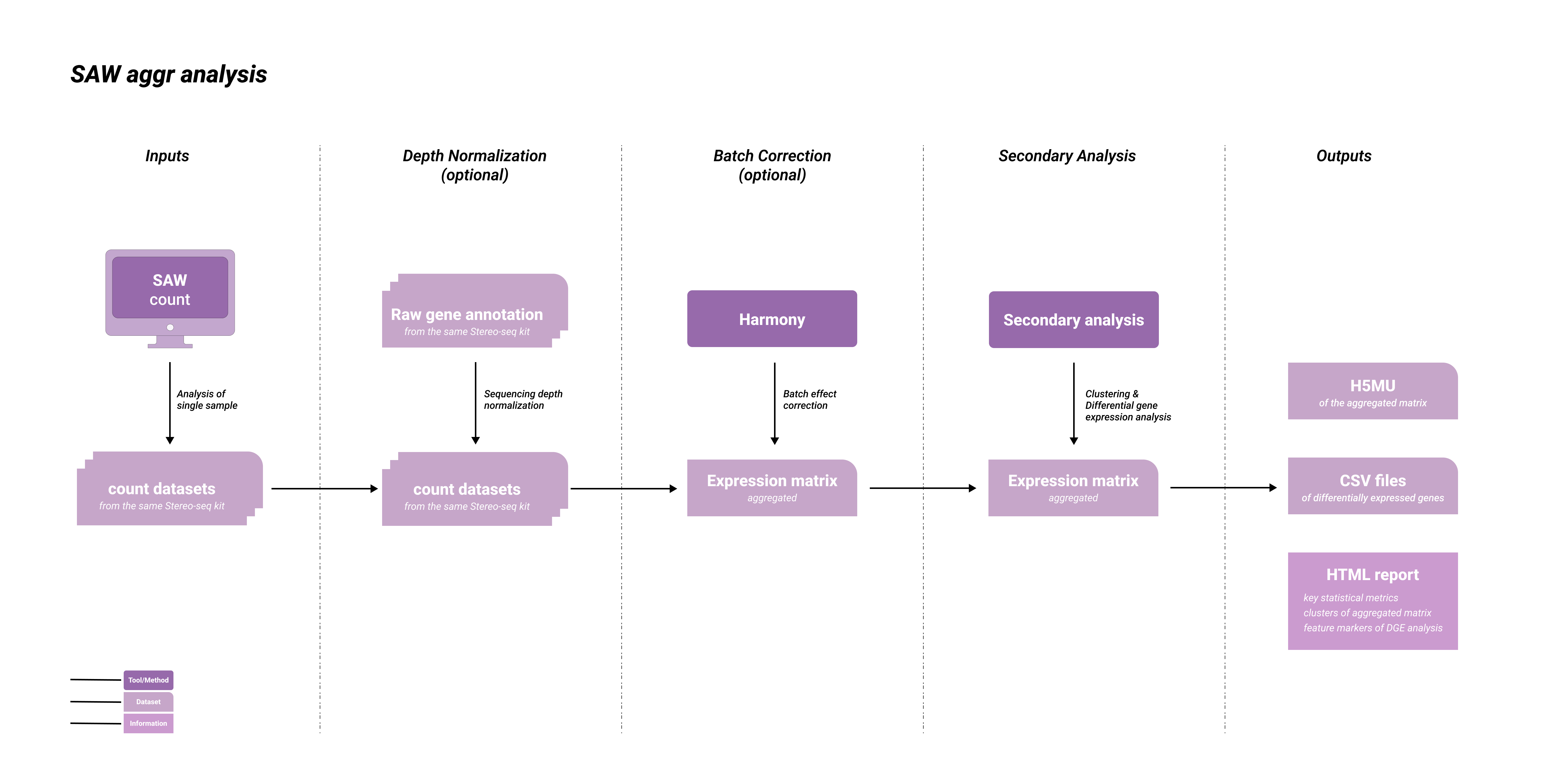
为了满足上述需求,SAW aggr 分析流程被设计用于整合多次 saw count 运行生成的分析结果。该工作流会生成一个整合的数据集,对于以下环节至关重要:
- 测序深度归一化 (Sequencing depth normalization): 校正不同样本间测序深度的差异
- 批次效应校正 (Batch effect correction): 整合数据以消除技术噪音,即批次效应,同时保留生物学异质性
- 比较分析 (Comparative analysis): 支持基于分组的聚类和差异基因表达分析,以揭示特定条件下的生物学特征
工作流程图如下所示:
SAW aggr 流程不适用于以下场景:
- 试剂盒不兼容: 整合来自不同 Stereo-seq 试剂盒版本或检测类型的样本(例如,将 Stereo-seq T FF V1.2 与 Stereo-seq N FFPE V1.0 的样本混合),不同试剂盒条件可能会引入不同的技术特征和捕获效率,标准批次校正算法无法有效地校正这些差异。
- 重测序数据: 合并同一张 Stereo-seq 芯片(相同文库)的多次测序运行数据以增加 Read 深度。对于这种情况,请将来自不同批次的所有 FASTQ 文件提供给单样本分析流程
saw count进行处理。
前置条件
与从原始测试 FASTQ 文件开始的 saw count 流程不同,saw aggr 需要使用上游分析(saw count)输出的分析文件。
为了顺利运行 SAW aggr 流程,需要准备:
- 完成 SAW count 分析: 确保每个样本都已经成功运行了
saw count流程。 - 准备元数据: 明确实验设计信息,例如,哪些样本属于“对照组(Control)”,哪些属于“处理组 (Treated)”。
配置文件 CSV
CSV 配置文件 (--slice-csv) 提供了每个样本的详细信息,它是数据加载、归一化和分组分析的核心控制文件。
slice_visual_file: (必选) 指定每个样本saw count运行生成的visualization.tar.gz或visualization.tar的文件路径。reads_info: (可选) 记录每个样本注释基因的原始比对 reads 数,对应saw count输出目录./outs/feature_expression/下的<SN>_raw_barcode_gene_exp.txt或<SN>_raw_barcode_gene_exp.txt.gz,流程使用这些值来计算测序深度归一化的因子。<group_name>(s): (可选) 定义生物学条件(例如,疾病组 vs 对照组),虽然文件可以包含多个分组列,但在下游分析中,只有被指定列会被用于分组差异表达分析。
如何指定分组: 使用 --deg-group-by=<column_name> 参数告诉流程具体使用哪一列来定义比较组。例如,设置 --deg-group-by='treatment' 将基于 "treatment" 列执行差异分析,而忽略 "timePoint" 等其他列信息。
输入配置 CSV 示例:
slice_visual_file,reads_info,<group1_name>,<group2_name>...
/path/to/task1/outs/visualization.tar,/path/to/task1/outs/feature_expression/sn1_raw_barcode_gene_exp.txt.gz,<condition1>,<conditionA>,...
/path/to/task2/outs/visualization.tar,/path/to/task2/outs/feature_expression/sn2_raw_barcode_gene_exp.txt.gz,<condition2>,<conditionB>,...
配置 CSV 文件中指定的文件路径(例如: slice_visual_file 和 reads_info 列)需为绝对路径(例如: /full/path/to/...)。
多样本分组配置示例
在多样本联合分析中(例如:有 4 个样本),填写分组信息的关键在于根据您的实验设计(Experimental Design)来定义列名和对应的值。可以自由添加一列或多列来自定义分组属性:
场景一:标准的“处理组 vs 对照组”(两组对比) 假设您的 4 个样本中,2 个属于对照组(Control),2 个属于疾病处理组(Case)。您只需添加一个分组列(例如命名为 group):
slice_visual_file,reads_info,group
/path/to/sample1/outs/visualization.tar.gz,/path/to/sample1/outs/feature_expression/sample1_raw_barcode_gene_exp.txt,control
/path/to/sample2/outs/visualization.tar.gz,/path/to/sample2/outs/feature_expression/sample2_raw_barcode_gene_exp.txt,control
/path/to/sample3/outs/visualization.tar.gz,/path/to/sample3/outs/feature_expression/sample3_raw_barcode_gene_exp.txt,case
/path/to/sample4/outs/visualization.tar.gz,/path/to/sample4/outs/feature_expression/sample4_raw_barcode_gene_exp.txt,case
场景二:复杂的多因素设计(如:不同时期 + 不同药物处理) 假设您的 4 个样本涉及两个实验变量:不同的时间点(Day 1 和 Day 7)以及不同的给药情况(Vehicle 溶剂组 和 Drug 给药组)。您可以同时添加多个自定义列(例如 timePoint 和 treatment):
slice_visual_file,reads_info,timePoint,treatment
/path/to/sample1/outs/visualization.tar.gz,/path/to/sample1/outs/feature_expression/sample1_raw_barcode_gene_exp.txt,day1,vehicle
/path/to/sample2/outs/visualization.tar.gz,/path/to/sample2/outs/feature_expression/sample2_raw_barcode_gene_exp.txt,day3,drug
/path/to/sample3/outs/visualization.tar.gz,/path/to/sample3/outs/feature_expression/sample3_raw_barcode_gene_exp.txt,day7,vehicle
/path/to/sample4/outs/visualization.tar.gz,/path/to/sample4/outs/feature_expression/sample4_raw_barcode_gene_exp.txt,day7,drug
命令行
For a list of available parameters, simply type saw aggr --help. Set up the SAW aggr analysis command in your working directory:
如需获取可用参数的完整列表,只需在终端输入 saw aggr --help,在工作目录中输入 SAW aggr 分析命令:
cd /saw/runs

saw aggr \
    --id=<task_id> \
    --slice-csv=/path/to/configuration/csv \
    --bin-size=50 \
    --deg-group-by=group_name

##  --skip-depth-normalization
##  --skip-batch-effect
核心参数简介:
| Parameter | Description |
|---|---|
--id <ID> | (Required, default to None) A unique task id ([a-zA-Z0-9_-]+) which will be displayed as the output folder name and the title of HTML report. It is required for saw aggr analysis. |
--slice-csv <CSV> | (Required, default to None) The input CSV file provides information for each slice, usually containing a column named If the column Group columns |
--bin-size <INT> | (Optional, default to 50) An appropriate bin size for the analysis aggregates multiple slices. Both sizes of square binning and cellbin (--bin-size=cell) are accepted. |
--skip-depth-normalization | (Optional, default to None) Force skip sequencing depth normalization between slices. By default, if the input --slice-csv contains a reads_info column, the pipeline normalizes sequencing depth across samples. If the column is missing, normalization is skipped automatically. |
--skip-batch-correction | (Optional, default to None) Whether to skip the batch effect correction, used to integrate data from multiple slices. Batch effect correction is essential when slices are processed in different batches, at different times, or with other technical variations that can introduce systematic, non-biological differences. |
--intersect-genes | (Optional, default to None) Whether to retain only the intersecting genes present in all slices; otherwise, retain the union of all genes. When used, the pipeline performs an intersection of genes. The final combined matrix includes only those genes present in every sample. When not used (the default setting), the pipeline performs a union of all genes present across the samples. The final combined matrix includes every gene found in any sample, with missing values filled with zeros for samples where a gene was not detected. |
--deg-group-by <TEXT> | (Optional, default to None) Specify a column name from If none are specified, the workflow will skip the inter-group analysis. |
--Leiden-resolution <FLOAT> | (Optional, default to 1.0) The resolution parameter controls the coarseness of the clustering when performing Leiden on integrated multiple slices. Higher values lead to more clusters. |
--deg-test-method <TEXT> | (Optional, default to t_test) Specify the statistical method for differential gene expression analysis. Supported options include t_test and wilcoxon_test. The selected method will be applied to all comparisons in the workflow. |
--p-adjust-method <TEXT> | (Optional, default to benjamini-hochberg) Specify the multiple testing correction method for p-value adjustment in differential gene expression analysis. Supported options: benjamini-hochberg, bonferroni. |
--output <PATH> | (Optional, default to None) Output directory. |
--gpu-id <NUM> | (Optional, default to -1) Set GPU id, according to GPU resources in the computing environment. Default to -1, which means running the pipeline using the CPU. |
基因特征信息
在加载多样本数据时,SAW aggr 通过以下两种策略之一建立统一的基因特征空间:
- 取并集 (Union)(默认):保留出现在任何样本中的基因,有助于保留可能仅在特定样本或条件下表达的罕见基因。
- 取交集 (Intersect)(使用
--intersect-genes):仅保留所有样本中共有的基因,对于消除因批次间捕获效率差异引起的噪音有用。
深度归一化 (Depth normalization)
为了减轻由测序深度或捕获效率不同而引发的系统性差异,流程默认执行测序深度归一化。
- 默认处理:根据每个输入样本的原始基因表达记录(总 MID 计数)计算归一化因子,将所有样本拉平至具有可比性的测序深度。
- 跳过归一化(使用
--skip-depth-normalization):如果希望保留原始的测序深度差异,或计划稍后执行自定义归一化,可跳过此步骤。
saw count 目录下 ./outs/feature_expression/ 中的 <SN>_raw_barcode_gene_exp.txt 或其压缩包包含了用于深度归一化的坐标、基因、MID 及 reads 的计数信息。
批次效应校正 (Batch effect correction)
SAW aggr 为数据整合提供了灵活的策略:
- 默认处理 (Harmony 算法):流程自动采用 Harmony 算法校正批次效应,可以在保留生物学异质性的同时,对齐跨样本中相同的细胞类型。
- 跳过校正(使用
--skip-batch-correction):如果希望观察原始的技术差异,或者样本在生物学上完全互斥(例如,不存在共享细胞类型的不同组织),可以选择跳过此步骤。
运行 SAW aggr
Scenario in this tutorial, we will perform a joint analysis of two mouse brain sections (C04042E2 and C04042E3)to demonstrate the SAW aggr analysis. These two are officiald released demo datasets, download them from our database.
在本教程场景中,我们将对两个小鼠大脑切片(C04042E2 和 C04042E3)进行多片联合分析,以演示 SAW aggr 的使用。这是两个官方发布的演示数据集,可从时空数据库下载。
cd /saw/runs

saw aggr \
    --id=mouse_brain_bin50_compare \
    --slice-csv=./configuration.csv \
    --bin-size=50 \
    --deg-group-by="group"

##  --skip-depth-normalization
##  --skip-batch-effect
示例配置 CSV:
slice_visual_file,reads_info,group
/path/to/C04042E2/outs/visualization.tar.gz,/path/to/C04042E2/outs/feature_expression/C04042E2_raw_barcode_gene_exp.txt,case
/path/to/C04042E3/outs/visualization.tar.gz,/path/to/C04042E3/outs/feature_expression/C04042E3_raw_barcode_gene_exp.txt,control
探索输出目录
流程分析完成后,您的工作目录中将出现一个名为 mouse_brain_bin50_compare(由 --id 参数指定)的新文件夹。
SAW aggr 生成的所有元数据和输出文件结构如下:
mouse_brain_bin50_compare
├── pipeline-logs
├── STEREO_ANALYSIS_WORKFLOW_PROCESSING
└── outs
    ├── analysis
    ├── <id>.report.html
    └── visualization.tar
.png)
进一步探究流程输出结果 :
- 跳转至HTML报告解读;
- 熟悉
visualization.tar可视化文件; - 了解输出结果中的各种文件类型。